Intro
REopt® optimization happens during the post-processing of each scenario. Refer to the Getting Started page for instructions on creating and running building energy models.
CLI commands are used to run and post-process each scenario, and onscreen help is always available with uo --help.
Also note that two types of REopt optimization are available:
- scenario-level, which optimizes for the aggregate load of the entire district being simulated, and
- feature-level, which optimizes each building’s load individually.
You may chose to optimize by one or both of these approaches according to your project objectives.
Workflow
REopt Optimization Assumption Files
In your URBANopt project directory, you should see two example REopt assumption files in a reopt folder (base_assumptions.json and multiPV_assumptions.json). If the reopt folder is missing, first create a new baseline REopt-enabled ScenarioFile with the uo create --scenario-file command (type uo create --help for usage help). These files follow the format outlined in the API documentation and can be customized to your specific project needs. Though CLI commands, they will be updated with basic information from your Feature and Scenario Reports (i.e. latitude, longitude, electric load profile) and submitted to the REopt API.
In particular, you will want to make sure that the urdb_label in the assumptions file maps to a suitable utility rate label from the URDB. The label is the last term of the URL of a utility rate detail page (i.e. the label for the rate at https://openei.org/apps/IURDB/rate/view/5b0d83af5457a3f276733305 is 5b0d83af5457a3f276733305).
Also note that the example reopt/multiPV_assumptions.json file contains an array of PV inputs to allow for the optimization of multiple PV systems at once.
Lots of detail can be specified by customizing the REopt assumptions file. Some examples:
- To simulate an off-grid scenario: change
off_grid_flagtotrue. - To set min/max renewable fraction of power in a district: change
renewable_electricity_min_pctand/orrenewable_electricity_max_pctto a value between 0-1, where 0 is 0% renewable and 1 is 100% renewable. Max renewable can be larger than 1 if more energy is produced than consumed.
REopt Time Series Resolution
The REopt time series resolution is controlled by the Scenario time_steps_per_hour setting in the assumptions file, and can be different than the Scenario or Feature Report resolution resulting from the OpenStudio simulation (and recorded in the CSV). Note that resolutions that are not evenly divisible by each other (i.e. 7 time steps per hour into 4 per hour) may cause unexpected results or errors due to rounding errors. If a REopt resolution is not defined in the assumptions file, the recommended resolution of 1 per hour is used.
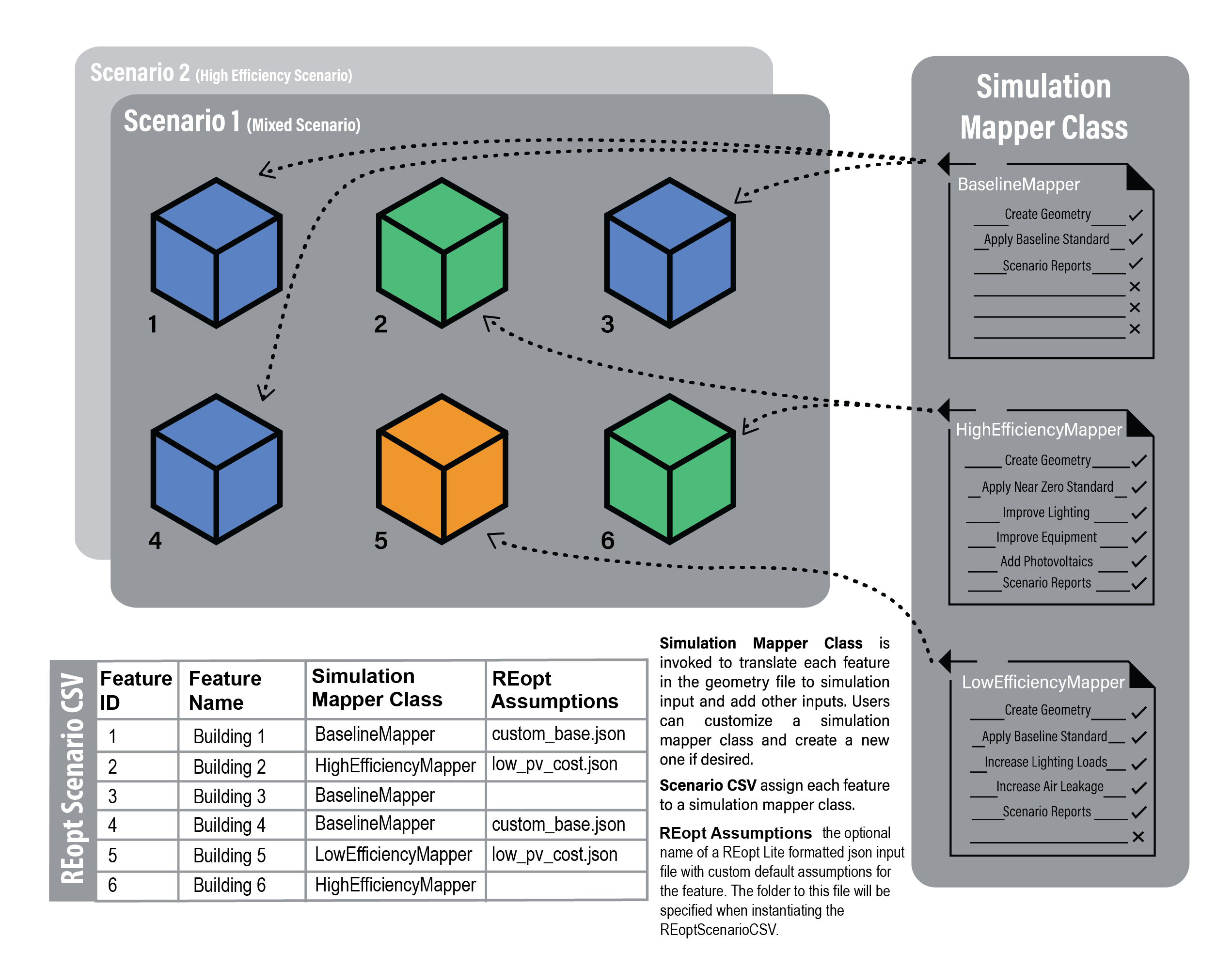
Mapping REopt Assumption Files to Features
In your Scenario File enabled for REopt you will see a REopt Assumptions column. Before post-processing ensure that each feature has the appropriate assumptions file specified in this CSV file.
The following figure represents how Simulation Mapper Classes can be assigned to different Features from the FeatureFile in the Scenario CSV.
Running REopt
The type of optimization is specified in the CLI call:
The --reopt-scenario command allows you to post-process a ScenarioReport in aggregate. This is suitable for community-scale optimizations.
uo process --reopt-scenario --feature <path/to/FEATUREFILE.json> --scenario <path/to/SCENARIOFILE.csv>
The --reopt-scenario-assumptions-file option can be used with this command to specify the assumptions file to use. If omitted, the base_assumptions.json file from the reopt folder will be used, as described above.
Alternatively, The --reopt-feature command allows you to post-process a Scenario for each of its Feature Reports before aggregating into a summary in the Scenario Report. This runs REopt optimization on each building individually. The assumptions file to use for each feature should be specified in the REopt-enabled ScenarioCSV file.
uo process --reopt-feature --feature <path/to/FEATUREFILE.json> --scenario <path/to/REOPT_SCENARIOFILE.csv>
Understanding REopt Results
After REopt post-processing, you will find that the new ScenarioReport contains updated distributed_generation and timeseries_CSV attributes.
Distributed Generation Updates
The following provides an example of distributed_generation attributes that have been updated by post-processing with REopt.
  "distributed_generation": {
      #optimal lifecycle costs
      "lcc_us_dollars": 30943,
      #business as usual lifecycle costs
      "lcc_bau_us_dollars": 40040.0,
      #optimal net present value
      "npv_us_dollars": 9097.0,
      #optimal costs paid to the utility for energy charges, year 1
      "year_one_energy_cost_us_dollars": 750.3,
      #optimal costs paid to the utility for demand charges, year 1
      "year_one_demand_cost_us_dollars": 0.0,
      #optimal total costs paid to the utility
      "year_one_bill_us_dollars": 1521.66,
      #optimal costs paid to the utility for demand charges, lifetime
      "total_demand_cost_us_dollars": 0.0,
      #optimal costs paid to the utility for energy charges, lifetime
      "total_energy_cost_us_dollars": 7189.5,
      #business as usual costs paid to the utility for energy charges, year 1
      "year_one_energy_cost_bau_us_dollars": 3407.27,
      #business as usual costs paid to the utility for demand charges, year 1
      "year_one_demand_cost_bau_us_dollars": 0.0,
      #business as usual total costs paid to the utility
      "year_one_bill_bau_us_dollars": 4178.63,
      #business as usual costs paid to the utility for energy charges, lifetime
      "total_energy_cost_bau_us_dollars": 32649.02,
      #business as usual costs paid to the utility for demand charges, lifetime
      "total_demand_cost_bau_us_dollars": 2189.75,
      #total optimal solar PV
      "total_solar_pv_kw": 0.0,
      #min outage duration system can sustain
      "resilience_hours_min": 3.0,
      #max outage duration system can sustain
      "resilience_hours_max": 6116.0,
      #average outage duration system can sustain
      "resilience_hours_avg": 0.0,
      #probability of surviving an outage by timestep
      "probs_of_surviving":
        [ 0.0027, 0.0027,...condensing full response... ,0.0027],
      #probability of surviving an outage by month
      "probs_of_surviving_by_month":
        [ 0.0027, 0.0027...condensing full response...0.0027],
      #probability of surviving an outage by hour of day
      "probs_of_surviving_by_hour_of_the_day":
        [ 0.0027, 0.0027...condensing full response...0.0027],
      #list of all optimal solar PV systems
      "solar_pv": [
        {"size_kw": 8.0124}
      ],
      #list of all optimal wind systems
      "wind": [],
      #list of all optimal generator systems
      "generator": [],
      #list of all optimal battery storage systems
      "storage": [
        {"size_kw": 2.1848, "size_kwh": 4619}
      ]
    },
      }
Note that the solar_pv, wind, generator and storage arrays will contain lists of all economic technologies across all features. For example, if solar PV is economic for two Feature Reports then the solar_pv array will contain these two capacities. Moreover, the total capacity of both systems will be recorded in the total_solar_pv_kw attribute. Also, note that the attributes in distributed_generation containing “bau” in the name are business as usual metrics that can be used to understand the relative economic attactiveness of the optimal solution.
Timeseries CSV Updates
After REopt post-processing, you will also find that ScenarioReport timeseries_CSV contains the following new optimal dispatch fields:
| new column name | unit |
|---|---|
| REopt:ElectricityProduced:Total(kW) | kW |
| REopt:Electricity:Load:Total(kW) | kW |
| REopt:Electricity:Grid:ToLoad(kW) | kW |
| REopt:Electricity:Grid:ToBattery(kW) | kW |
| REopt:Electricity:Storage:ToLoad(kW) | kW |
| REopt:Electricity:Storage:ToGrid(kW) | kW |
| REopt:Electricity:Storage:StateOfCharge(kW) | kW |
| REopt:ElectricityProduced:Generator:Total(kW) | kW |
| REopt:ElectricityProduced:Generator:ToBattery(kW) | kW |
| REopt:ElectricityProduced:Generator:ToLoad(kW) | kW |
| REopt:ElectricityProduced:Generator:ToGrid(kW) | kW |
| REopt:ElectricityProduced:PV:Total(kW) | kW |
| REopt:ElectricityProduced:PV:ToBattery(kW) | kW |
| REopt:ElectricityProduced:PV:ToLoad(kW) | kW |
| REopt:ElectricityProduced:PV:ToGrid(kW) | kW |
| REopt:ElectricityProduced:Wind:Total(kW) | kW |
| REopt:ElectricityProduced:Wind:ToBattery(kW) | kW |
| REopt:ElectricityProduced:Wind:ToLoad(kW) | kW |
| REopt:ElectricityProduced:Wind:ToGrid(kW) | kW |
NOTE: A REopt solution may contain multiple PV systems. In this case the aggregate generation from all PV systems will be reported in the PV columns.
Additional Outputs
REopt API responses are saved in reopt folders. This information may be helpful in interpreting results or debugging errors (i.e. identifying if API rate-limits have been reached).
If you post-processed with --reopt-scenario the reopt folder will be at the top level of scenerio in the run (i.e. run\reopt_scenario\reopt). Otherwise, if you run with --reopt-feature each feature will have its own reopt folder (i.e. run\reopt_scenario\1\reopt).
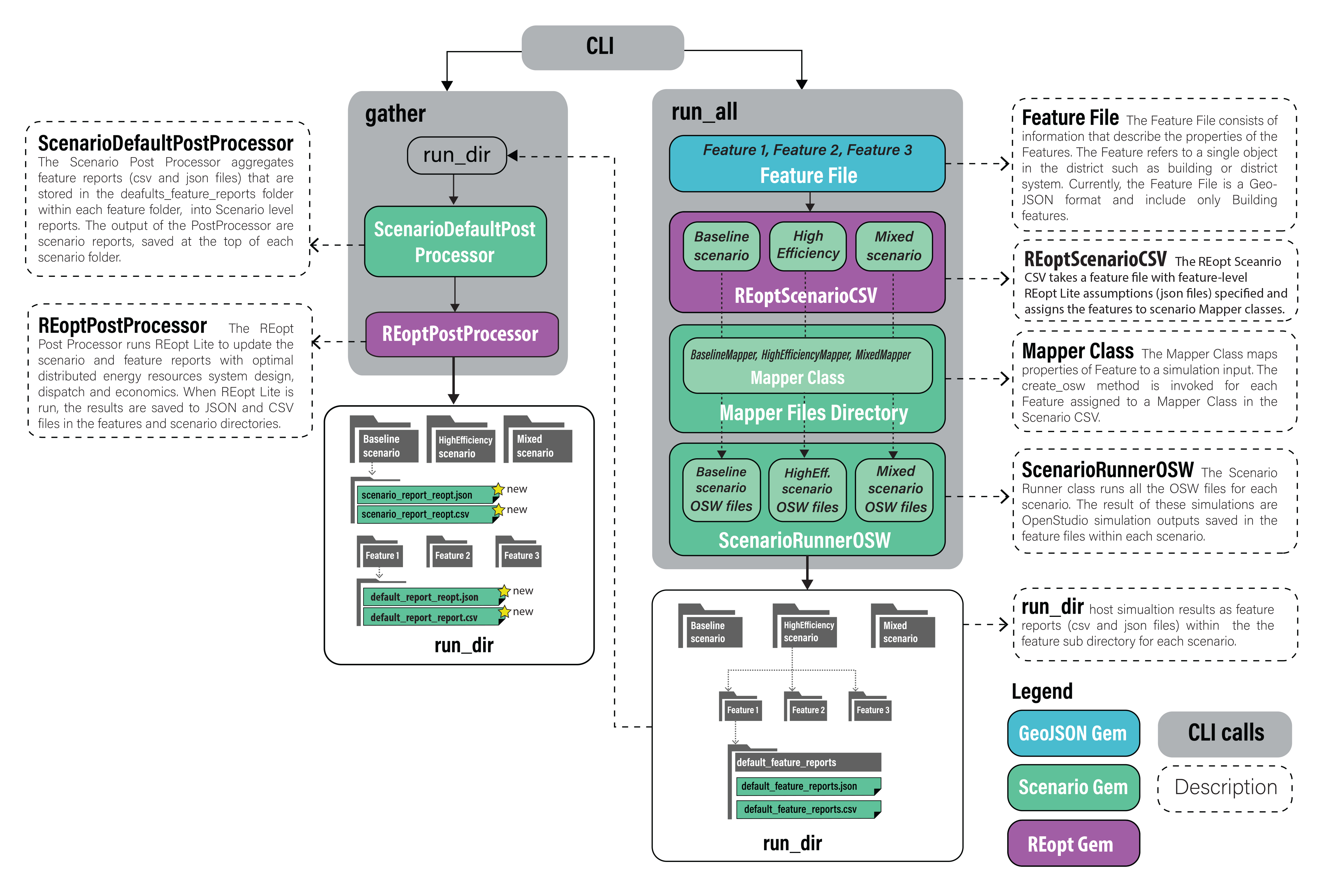
Additional Information
The figure below describes the workflow that takes place on implementing the run and process CLI commands.